
Cycling Analytics
This is an analysis I did back in 2020 which was recently updated to included new data up to April 2022. Please check it out and compare it to my trading algorithm which implements more programming best practices.
Cycling is one of my favorite pastimes and at one point I wanted to go professional. Now that those days are over, and a new interest in programming has over come me, I wanted to blend the two in a fun and simple project. Luckily, ever since I was 14 I uploaded all my rides to a website called Strava, which allows you to collect old data with a data dump. The following is an analysis of the last 10 years of my cycling journey.
Converting the data into a workable format
First off, the data for this project was downloaded manually from Strava as a zip file. In the zip file were many folders with one containing all the rides with non-descript names in either a .fit or .gpx file. .fit files are proprietary to Garmin tracking devices and are the only relevant files for this project. It contains GPS data information along with data coming from connected sensors like a heart rate monitor.
Since I wanted to learn a bit of python and bash scripting, I found a callable python script, modified it, and used it to convert all .fit files to .csv. Most of the credit must go to Max Candocia and his blog post.
import csv
import os
# to install fitparse, run
# sudo pip3 install -e git+https://github.com/dtcooper/python-fitparse#egg=python-fitparse
import fitparse
import pytz
from copy import copy

# for general tracks
allowed_fields = ['timestamp', 'position_lat', 'position_long', 'distance',
                  'enhanced_altitude', 'altitude', 'enhanced_speed',
                  'speed', 'heart_rate', 'cadence', 'fractional_cadence',
                  'temperature']
required_fields = ['timestamp', 'position_lat', 'position_long', 'altitude']

# for laps
lap_fields = ['timestamp', 'start_time', 'start_position_lat', 'start_position_long',
              'end_position_lat', 'end_position_long', 'total_elapsed_time', 'total_timer_time',
              'total_distance', 'total_strides', 'total_calories', 'enhanced_avg_speed', 'avg_speed',
              'enhanced_max_speed', 'max_speed', 'total_ascent', 'total_descent',
              'event', 'event_type', 'avg_heart_rate', 'max_heart_rate',
              'avg_running_cadence', 'max_running_cadence',
              'lap_trigger', 'sub_sport', 'avg_fractional_cadence', 'max_fractional_cadence',
              'total_fractional_cycles', 'avg_vertical_oscillation', 'avg_temperature', 'max_temperature']
# last field above manually generated
lap_required_fields = ['timestamp', 'start_time', 'lap_trigger']

# start/stop events
start_fields = ['timestamp', 'timer_trigger', 'event', 'event_type', 'event_group']
start_required_fields = copy(start_fields)
#
all_allowed_fields = set(allowed_fields + lap_fields + start_fields)

UTC = pytz.UTC
CST = pytz.timezone('US/Central')

# files beyond the main file are assumed to be created, as the log will be updated only after they are created
ALT_FILENAME = True
ALT_LOG = 'file_log.log'


def read_log():
    with open(ALT_LOG, 'r') as f:
        lines = f.read().split()
    return lines


def append_log(filename):
    with open(ALT_LOG, 'a') as f:
        f.write(filename)
        f.write('\n')
    return None


def main():
    files = os.listdir()
    fit_files = [file for file in files if file[-4:].lower() == '.fit']
    if ALT_FILENAME:
        if not os.path.exists(ALT_LOG):
            os.system('touch %s' % ALT_FILENAME)
            file_list = []
        else:
            file_list = read_log()
    for file in fit_files:
        if ALT_FILENAME:
            if file in file_list:
                continue
        new_filename = file[:-4] + '.csv'
        if os.path.exists(new_filename) and not ALT_FILENAME:
            # print('%s already exists. skipping.' % new_filename)
            continue
        fitfile = fitparse.FitFile(file,
                                   data_processor=fitparse.StandardUnitsDataProcessor())

        print('converting %s' % file)
        write_fitfile_to_csv(fitfile, new_filename, file)
    print('finished conversions')


def lap_filename(output_filename):
    return output_filename[:-4] + '_laps.csv'


def start_filename(output_filename):
    return output_filename[:-4] + '_starts.csv'


def get_timestamp(messages):
    for m in messages:
        fields = m.fields
        for f in fields:
            if f.name == 'timestamp':
                return f.value
    return None


def get_event_type(messages):
    for m in messages:
        fields = m.fields
        for f in fields:
            if f.name == 'sport':
                return f.value
    return None


def write_fitfile_to_csv(fitfile, output_file='test_output.csv', original_filename=None):
    messages = fitfile.messages
    data = []
    lap_data = []
    start_data = []
    if ALT_FILENAME:
        # this should probably work, but it's possibly
        # based on a certain version of the file/device
        timestamp = get_timestamp(messages)
        event_type = get_event_type(messages)
        if event_type is None:
            event_type = 'other'
        output_file = event_type + '_' + timestamp.strftime('%Y-%m-%d_%H-%M-%S.csv')
    for m in messages:
        skip = False
        skip_lap = False
        skip_start = False
        if not hasattr(m, 'fields'):
            continue
        fields = m.fields
        # check for important data types
        mdata = {}
        for field in fields:
            if field.name in all_allowed_fields:
                if field.name == 'timestamp':
                    mdata[field.name] = UTC.localize(field.value).astimezone(CST)
                else:
                    mdata[field.name] = field.value
        for rf in required_fields:
            if rf not in mdata:
                skip = True
        for lrf in lap_required_fields:
            if lrf not in mdata:
                skip_lap = True
        for srf in start_required_fields:
            if srf not in mdata:
                skip_start = True
        if not skip:
            data.append(mdata)
        elif not skip_lap:
            lap_data.append(mdata)
        elif not skip_start:
            start_data.append(mdata)
    # write to csv
    # general track info
    with open(output_file, 'w') as f:
        writer = csv.writer(f)
        writer.writerow(allowed_fields)
        for entry in data:
            writer.writerow([str(entry.get(k, '')) for k in allowed_fields])
    # lap info
    with open(lap_filename(output_file), 'w') as f:
        writer = csv.writer(f)
        writer.writerow(lap_fields)
        for entry in lap_data:
            writer.writerow([str(entry.get(k, '')) for k in lap_fields])
    # start/stop info
    with open(start_filename(output_file), 'w') as f:
        writer = csv.writer(f)
        writer.writerow(start_fields)
        for entry in start_data:
            writer.writerow([str(entry.get(k, '')) for k in start_fields])
    print('wrote %s' % output_file)
    print('wrote %s' % lap_filename(output_file))
    print('wrote %s' % start_filename(output_file))
    if ALT_FILENAME:
        append_log(original_filename)


if __name__ == '__main__':
    main()
Then when calling the following bash script in the command line it unzips the compressed .fit files and converts them to .csv.
#!/bin/bash

# move to the activities directory
cd /Users/kylekent/Library/CloudStorage/Dropbox/cycling_analytics/strava_export_04-15-22/activities;
# unzip all the .fit.gz files
gzip -d *.fit.gz;
# run the py file to convert all the fit files to csv
python3 fit2csv.py;
Loading the data in python
Now that the GPS data is in a .csv format we can load it into python for processing. The following script loads file names into a list, creates a function to iterate over the list and appends the data into one pandas dataframe. Other relevant variables are calculated in new columns.
import pandas as pd
import numpy as np
import os, glob
import re

# getting a list of files
csv_files = []
os.chdir('/Users/kylekent/Desktop/research/CS_misc/GitHub/strava_project/strava_export_10-13-20/activities/')
for file in glob.glob('*.csv'):
    csv_files.append(file)
# now lets organize them by date with the newest rides coming first
csv_files = sorted(csv_files, key = str.lower, reverse = True)

# here's a function to get all the files loaded into a df
def get_csv_files():
    # getting csv file names
    csv_files = []
    os.chdir('/Users/kylekent/Desktop/research/CS_misc/GitHub/strava_project/strava_export_10-13-20/activities/')
    for file in glob.glob('*.csv'):
        csv_files.append(file)
    # ordering the list
    csv_files = sorted(csv_files, key=str.lower, reverse=True)
    # setting up the df
    col_names = ['timestamp', 'position_lat', 'position_long', 'distance', 'enhanced_altitude', 'altitude', 'enhanced_speed', 'speed', 'heart_rate', 'cadence', 'fractional_cadence', 'temperature', 'file_index']
    df = pd.DataFrame(columns = col_names)
    for i in range(len(csv_files)):
        f = open(csv_files[i], 'r')
        dft = pd.read_csv(f)
        dft['file_index'] = i
        df = df.append(dft)
        f.close()
    # resetting the index
    df = df.reset_index(drop=True)
    return df

# calling the function
all_rides = get_csv_files()
A few columns need to be added that will help our analyses, specifically time variables but also conversions of the raw data into more readable formats. The following code chunk creates time columns, calculates things like speed and elevation gain, then writes the dataframe to a new compressed .csv.gz file. This is the file that will be used to plot the GPS data.
# adding date columns
all_rides['timestamp'] = pd.to_datetime(all_rides['timestamp'], utc = True).dt.tz_convert(tz = 'America/Chicago')
all_rides['date'] = pd.to_datetime(all_rides['timestamp'].dt.strftime('%Y-%m-%d'))
all_rides['year'] = all_rides['timestamp'].dt.strftime('%Y')
all_rides['month'] = all_rides['timestamp'].dt.strftime('%m')

# getting variables to compare speed and elevation
avg_speed = all_rides.groupby('file_index', as_index = False)['enhanced_speed'].mean()
avg_speed.columns.values[1] = 'avg_speed'

all_rides = all_rides.join(avg_speed, on = 'file_index', rsuffix = '_del')
del df_2020['file_index_del']
del avg_speed

# writing the file
all_rides.to_csv('/Users/kylekent/Desktop/research/CS_misc/GitHub/strava_project/all_rides.csv.gz', index = False, compression = 'gzip')
Creating an aggregate dataset
The previous dataset containing all information on the bike rides is not necessary to compare descriptive stats between the rides. So the following code takes all the rides and boils them down into a wide dataset with each row having stats on only one ride. That file gets written to a .csv.gz so I can plot it in r.
all_rides_avgs = all_rides.groupby('file_index', as_index = False).agg({'elevation_gain':'sum', \
                                                                        'avg_speed':'mean', \
                                                                        'distance':'max', \
                                                                        'heart_rate': 'mean'})
all_rides_avgs['date'] = all_rides.groupby('file_index')['date'].unique()
all_rides_avgs['year'] = all_rides.groupby('file_index')['year'].unique()
all_rides_avgs['month'] = all_rides.groupby('file_index')['month'].unique()

all_rides_avgs.dtypes.apply(lambda x: x.name).to_dict()
all_rides_avgs.to_csv('/Users/kylekent/Desktop/research/CS_misc/GitHub/strava_project/all_rides_avgs2.csv.gz', index = False, compression = 'gzip')
Plotting rides with ggplot
Originally I planned to show interactive plots of a GPS heatmap for all my rides. Sadly, the files are too large for github pages. Instead the non-interactive heat maps are given below. If you’d like to see the interactive html files I am happy to share them with you.
To display the GPS data, the files from all my rides and the aggregate file were loaded into the r and plotted with ggplot. I forgot to convert a few of the units from metric to imperial and a few variables needed to be added to work with plotly. My choice of data formatting is to use data.tables because of its syntax and efficiency with large datasets.
library(ggplot2)
library(data.table)
library(plotly)
library(scales)
library(tidyverse)

# load in file
all.rides = as.data.table(read.csv('all_rides.csv.gz'))
avg.rides = as.data.table(read.csv('all_rides_avgs2.csv.gz'))

# modify them to fit data structures
all.rides[, timestamp := as.POSIXct(timestamp)]
all.rides[, `:=` (date = format(timestamp, '%Y-%m-%d'),
                  year = format(timestamp, '%Y'))]

# convert all metric to imperial measurments
all.rides[, `:=` (enhanced_speed = enhanced_speed*.62137,
           avg_speed = avg_speed*.62137,
           distance = distance*.62137,
           enhanced_altitude = enhanced_altitude*3.28084,
           elevation_change = elevation_change*3.28084,
           elevation_gain = elevation_gain*3.28084,
           avg_temp = temperature*(9/5)+32)]

# to create an interactive map some of the variables per ride need to have descriptive stat columns
all.rides[, `:=` (ride_distance = max(distance),
                  sum_elevation_gain = sum(elevation_gain, na.rm = T),
                  avg_temp = mean(temperature, na.rm = T),
                  duration = as.numeric((max(timestamp) - min(timestamp))/3600)),
          by = file_index]

avg.rides[, timestamp := all.rides[, mean(timestamp, na.rm = T)]] # seconds of the timestamp don't matter here to avging works
avg.rides[, `:=` (date = format(timestamp, '%Y-%m-%d'),
                  year = format(timestamp, '%Y'),
                  month = format(timestamp, '%m'),
                  day = format(timestamp, '%d'))]

avg.rides[, `:=` (timestamp = mean(timestamp, na.rm = T),
                          sum_elevation_gain = sum(elevation_gain, na.rm = T),
                          avg_speed = mean(enhanced_speed, na.rm = T),
                          ride_distance = max(distance),
                          duration = mean(duration, na.rm = T)),
                       by = file_index]
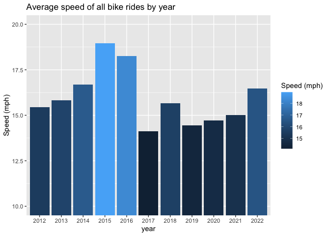
Ever since I started racing back in 2012 my passion for cycling took off. You can see that my average speed increased by year until I was 17 (in 2015) and at my peak performance but tapered off when I got injured in 2016 and went off to school without a pro contract. When in school I practically gave up riding due to depression, resentment, and a lack of enjoyement. Yet in 2018 as my depression subsided and I started coaching a junior cycling team which really got me into shape. That didn’t last long as my upper classmen years took hold and I began doing research giving me little freetime. Now as I have more free time out of school I am starting to race again and that is reflected in the speed of my rides.
# bar graph of avg speed per year
ggplot(avg.rides[avg_speed >= 5,.(speed = mean(avg_speed, na.rm = T)), year],
       aes(x = year, y = speed, fill = speed)) +
  geom_bar(stat = 'identity') +
  scale_y_continuous(limits = c(10, 20), oob = rescale_none) +
  labs(title = 'Average speed of all bike rides by year', fill = 'Speed (mph)') +
  ylab(label = 'Speed (mph)')
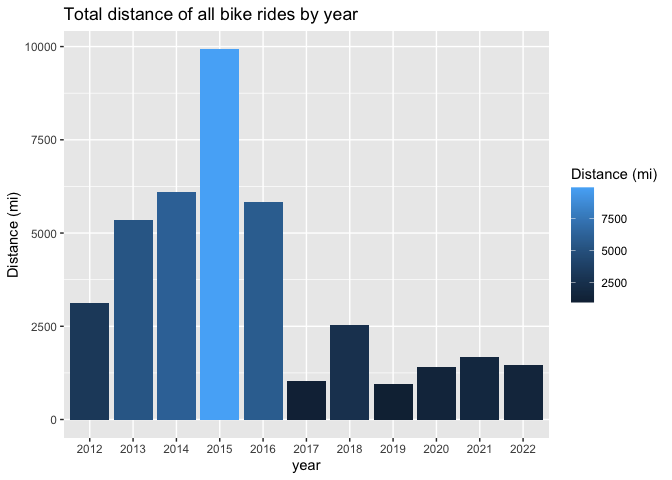
The same narrative arises when we look at my distance rode each year. A steady increase until 2015, then a drop during school. Although 2022 is set to be a good year as these data as presented are current up to April 15th, 2022.
# bargraph of distance per year
ggplot(avg.rides[,.(year_distance = sum(ride_distance, na.rm = T)), year],
       aes(x = year, y = year_distance, fill = year_distance)) +
  geom_bar(stat = 'identity') +
  labs(title = 'Total distance of all bike rides by year', fill = 'Distance (mi)') +
  ylab(label = 'Distance (mi)')
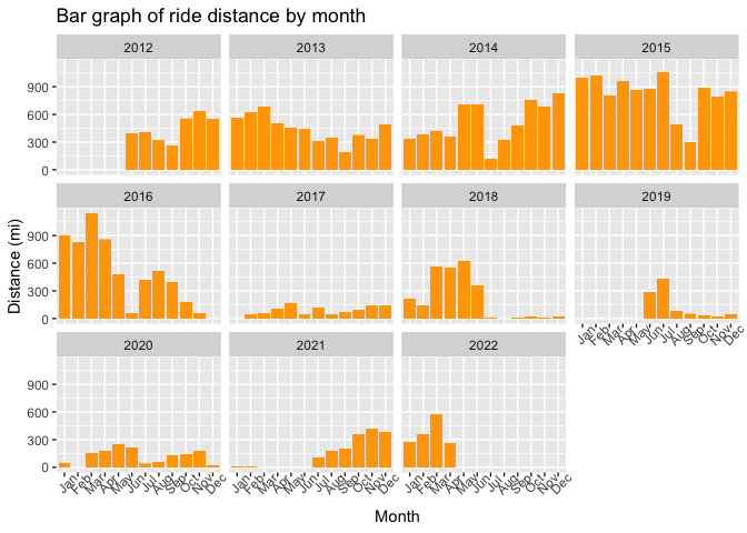
The following bargraph outlines how many miles I rode each month for every year that I have data on. There are clear peaks and troughs from 2012-2016 during specific times of the race season are present, or I am taking a break. Keep in mind I lived in Arizona so most of my rides occurred in the early part of the year and tapered during the summer.
# bargraph of distance per month over all the years
ggplot(avg.rides[, .(month_abr = format(timestamp, '%b'), ride_distance, year)][!is.na(month_abr)],
       aes(x = factor(month_abr, levels = c('Jan', 'Feb', 'Mar', 'Apr', 'May', 'Jun', 'Jul', 'Aug', 'Sep', 'Oct', 'Nov', 'Dec')),
           y = ride_distance)) +
  geom_bar(stat = 'identity', fill = 'orange') +
  theme(axis.text.x = element_text(angle = 45)) +
  facet_wrap(~year) +
  labs(title = 'Bar graph of ride distance by month') +
  xlab(label = 'Month') +
  ylab(label = 'Distance (mi)')
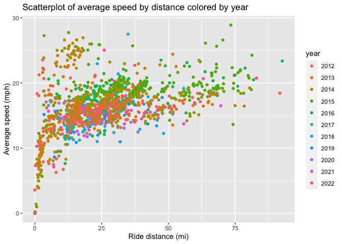
Another interesting relationship to analyze is the difference between the average speed of each ride by distance. I expected a curvilinear relationship where a few short rides (eg warming up for races) and long rides would have low average speeds. Turns out, as I got stronger my rides got faster and longer which is especially true for the 2015 rides. The longest rides tended to be the fastest because they were races, not training rides.
ggplot(avg.rides,
       aes(x = ride_distance, y = avg_speed, color = year)) +
  geom_point() +
  labs(title = 'Scatterplot of average speed by distance colored by year') +
  ylab('Average speed (mph)') +
  xlab('Ride distance (mi)')
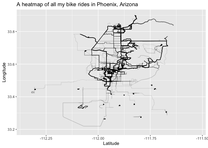
From 2012-2016 I lived in Scottsdale, Arizona so most of my riding happened around there. Below is a heat map of GPS data from those rides. You can see that most rides were loops, but some have low density strings that finish in high density loops. Those are races I rode to from home, did the race, then someone picked me up. If you hover over the images you can see some descriptive stats about each ride.
phx.heatmap <- ggplot(all.rides[(position_lat >= 33 & position_lat <= 35) & (position_long >= -113 & position_long <= -111)],
                      aes(x = position_lat, y = position_long,
                          group = file_index,
                          text = paste0('Date: ', date, '\n',
                                        'Distance(mi): ', round(ride_distance, 1), '\n',
                                        'Duration(hr): ', round(duration, 1), '\n',
                                        'Avg speed(mph): ', round(avg_speed, 1), '\n',
                                        'Elevation gain(ft): ', round(sum_elevation_gain)))) +
  geom_path(aes(group = file_index), alpha = .1) +
  xlim(33.2, 33.90) +
  ylim(-112.35, -111.525) +
  coord_flip() +
  labs(title = 'A heatmap of all my bike rides in Phoenix, Arizona') +
  xlab('Longitude') +
  ylab('Latitude')
# print regular plot
phx.heatmap
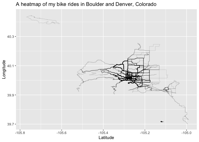
During my college years I lived in one of the best places to ride your bike in the country, Boulder, CO. These rides are less frequent but I still got out quite a bit and was able to explore other parts of Colorado like Denver.
CO.heatmap <- ggplot(all.rides[(position_lat >= 39 & position_lat <= 41) & (position_long >= -106 & position_long <= -104)],
                     aes(x = position_lat, y = position_long,
                         group = file_index,
                         text = paste0('Date: ', date, '\n',
                                       'Distance(mi): ', round(ride_distance, 1), '\n',
                                       'Duration(hr): ', round(duration, 1), '\n',
                                       'Avg speed(mph): ', round(avg_speed, 1), '\n',
                                       'Elevation gain(ft): ', round(sum_elevation_gain)))) +
  geom_path(aes(alpha = .1)) +
  xlim(39.7, 40.45) +
  ylim(-105.78, -104.99) +
  coord_flip() +
  labs(title = 'A heatmap of my bike rides in Boulder and Denver, Colorado') +
  xlab('Longitude') +
  ylab('Latitude')
CO.heatmap
I hope you enjoyed analyzing my bike rides with me and thank you for taking the time to do so!